Case studies
Here are some examples.
1. Ideal PSA simulation for green hydrogen production
In this example, pyAPEP.simide is used to simulate ideal PSA process for the separation of H2/N2 from the green ammonia.
Background
Because green ammonia is currently the favored transportation medium for carbon-free hydrogen, H2 separation and purification after the decomposition of NH3 is important to maximize the use of H2. Among all gas separation processes, the PSA is the most suitable process with the highest technological readiness. Therefore, this example compares adsorbents based on the performance of the ideal PSA for producing H2 from the N2/H2 gas mixture, and it determines the best adsorbent with the highest hydrogen recovery.
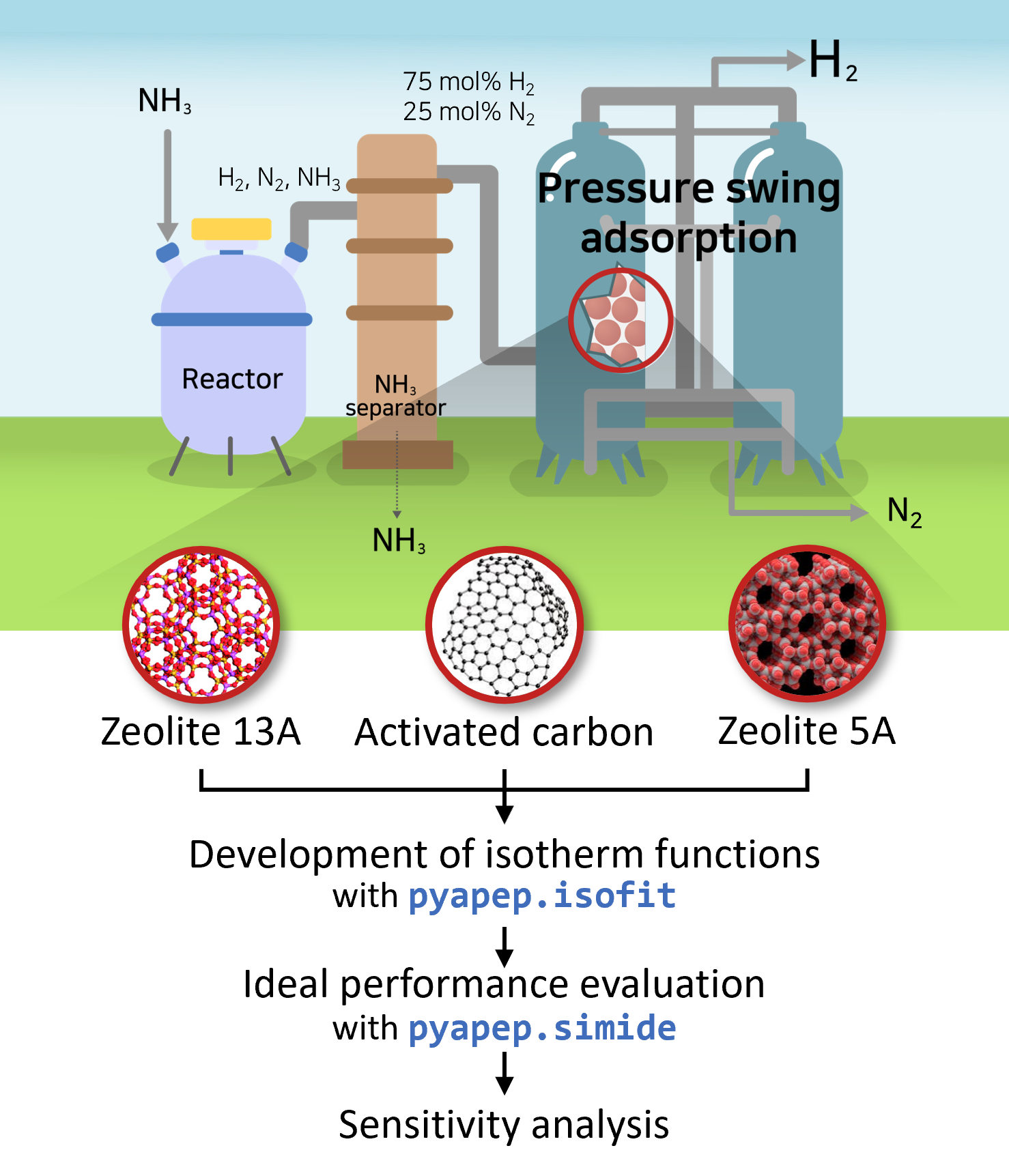
Figure. Schematic of pressure swing adsorption process used for H2 purification.
Process description
The target green ammonia decomposition process consists of an NH3 decomposition reactor, NH3 separator, and PSA process for H2 purification. In the NH3 decomposition reactor, the H2 was produced by decomposing NH3 into a mixture of N2 and H2. The NH3 separator removed residual NH3 from the feed stream. Therefore, the gas entering the target PSA process was assumed to be 25 mol% N2 and 75 mol% H2.
Goal
The goal of this example is the find best adsorbent among three adsorbents by comparing PSA perfomances. Adsorbent candidates are Zeolite 13X, 5A and activated carbon. All adsorbents and its pressure-uptake data could be found in literatures. This example contains isotherm fitting with given data(.csv), isotherm validation, development of mixture isotherm for each adsorbent, and ideal PSA simulation.
Before we start, import pyAPEP package and other python packages for data treatment and visualization. Also, users need to download the adsorption data files for three adsobents
# pyAPEP package import
import pyAPEP.isofit as isofit
import pyAPEP.simide as simide

# Data treatment package import
import numpy as np
import pandas as pd

# Data visualization package import
import matplotlib.pyplot as plt
Then, define pure isotherm function for hydrogen and nitrogen using pressure-uptake data samples. Before developing isotherm, users need to define or import datasets. If the isotherm parameters already exist, users can use those parameters by defining isotherm function manually.
# Data import
# adsorbent 1
Data_zeo13 = pd.read_csv('Casestudy1_Zeolite13X.csv')
# adsorbent 2
Data_ac = pd.read_csv('Casestudy1_Activated_carbon.csv')
# adsorbent 3
Data_zeo5 = pd.read_csv('Casestudy1_Zeolite5A.csv')

Data = [Data_zeo13, Data_ac, Data_zeo5]
# Find best isotherm function, Ideal PSA simulation
Adsorbent = ['Zeolite13X','Activated_carbon', 'Zeolite5A']
iso_pure = []
err_list = []
for i in range(3):
   ads = Data[i]

   P_N2 = ads['Pressure_N2 (bar)'].dropna().values
   q_N2 = ads['Uptake_N2 (mol/kg)'].dropna().values

   P_H2 = ads['Pressure_H2 (bar)'].dropna().values
   q_H2 = ads['Uptake_H2 (mol/kg)'].dropna().values

   N2_iso, _, _, N2_err = isofit.best_isomodel(P_N2, q_N2)
   H2_iso, _, _, H2_err = isofit.best_isomodel(P_H2, q_H2)

   iso_pure.append([N2_iso, H2_iso])
   err_list.append([N2_err, H2_err])

   # visualization
   plt.figure(dpi=70)
   plt.scatter(P_N2, q_N2, color = 'r')
   plt.scatter(P_H2, q_H2, color = 'b')

   P_max= max(max(P_N2), max(P_H2))
   P_dom = np.linspace(0, P_max, 100)
   plt.plot(P_dom, N2_iso(P_dom), color='r' )
   plt.plot(P_dom, H2_iso(P_dom), color='b' )

   plt.xlabel('Pressure (bar)')
   plt.ylabel('Uptake (mol/kg)')
   plt.title(f'{Adsorbent[i]}')
   plt.legend(['N$_2$ data', 'H$_2$ data',
             'N$_2$ isotherm','H$_2$ isotherm'], loc='best', fontsize=15)
   plt.show()
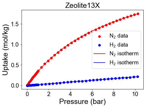
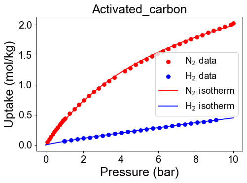
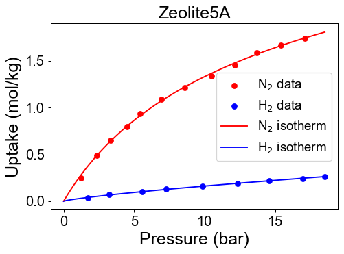
Check developed pure isotherm functions by comparing with raw data.
We need mixture isotherm functions to simulate PSA process. Here we define the hydrogen/nitrogen mixture isotherm functions with isofit.IAST
iso_mix_list = []
for i in range(3):
   N2_iso_ = lambda P,T: iso_pure[i][0](P)
   H2_iso_ = lambda P,T: iso_pure[i][1](P)

   iso_mix = lambda P,T : isofit.IAST([N2_iso_, H2_iso_], P, T)

   iso_mix_app = copy.deepcopy(iso_mix)
   iso_mix_list.append(iso_mix_app)
Then we need to define and run ideal PSA process.
results = []
for i in range(3):
   iso_mix = iso_mix_list[i]

   CI1 = simide.IdealColumn(2, iso_mix )

   # Feed condition setting
   P_feed = 8      # Feed presure (bar)
   T_feed = 293.15    # Feed temperature (K)
   y_feed = [1/4, 3/4] # Feed mole fraction (mol/mol)
   CI1.feedcond(P_feed, T_feed, y_feed)

   # Operating condition setting
   P_high = 8 # High pressure (bar)
   P_low  = 1 # Low pressure (bar)
   CI1.opercond(P_high, P_low)

   # Simulation run
   x_tail = CI1.runideal()
   R = 1- (y_feed[0]*(1-x_tail[0]))/(x_tail[0]*(1-y_feed[0]))
   print(R*100)       # Output: [x_H2, x_N2]
   results.append(R*100)
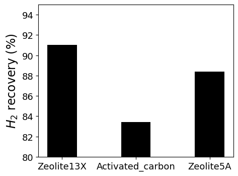
Now, we can calculate hydrogen recovery for this system. The results shows below. Finally, we found the best performance adsorbent.
# Results plot
Adsorbent = ['Zeolite13X','Activated_carbon', 'Zeolite5A']
plt.figure(dpi=100, figsize=(5, 4))
plt.bar(Adsorbent, results, width=0.4, color='black')
plt.ylim([80, 95])
plt.ylabel('H$_2$ recovery (%)', fontsize=17)
plt.yticks(fontsize=13)
plt.xticks( fontsize=13)
plt.show()
Additionally, sensitivity analysis was carried out. Below figure shows the results of sensitivity analysis for each variable using the developed PSA process model.
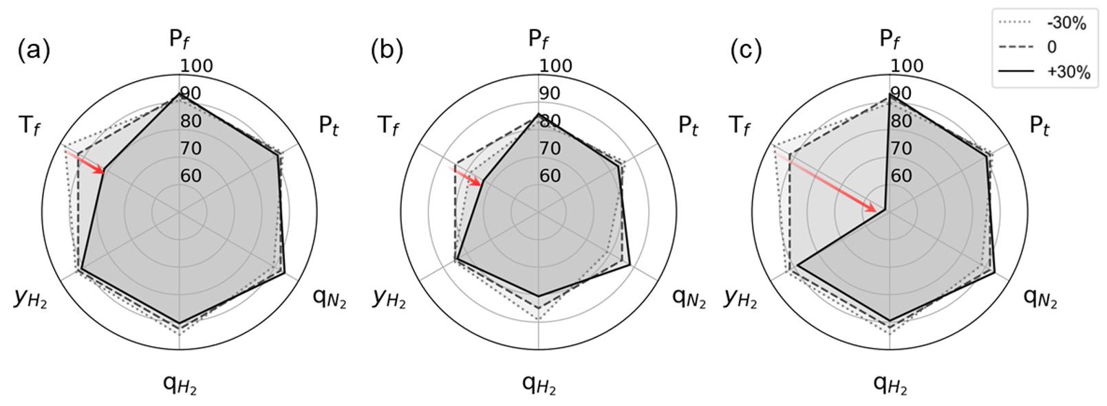
The left, center, and right columns show the results for zeolite 13X, activated carbon, and zeolite 5A. The results show the difference in H2 recovery for adsorption (\(P_{f}\)), regeneration pressure (\(P_{t}\)), temperature (\(T_{f}\)), and H2 composition (\(y_{H_2}\)) of the feed flow, and H2 and N2 uptake (\(q\)) were adjusted from -30 to +30%, respectively, while all other parameters were fixed. All three adsorbents reacted sensitively to H2 recovery according to the feed temperature, and in particular, in the case of zeolite 5A, when the temperature increased by 30 %, the H2 recovery rapidly decreased to approximately 50 %.
Below figure shows the H2 recovery for the five variables, except for the feed temperature, which further helped analyze the impact of other variables more clearly.

Although the degree of sensitivity for each adsorbent is different, the recovery increases with \(P_{f}\) and \(q_{N_2}\), and it tends to decrease as \(P_{t}\), \(y_{H_2}\) and \(q_{H_2}\) increase. Among all three adsorbents, \(T_{f}\) had the most significant impact H2 recovery, followed by \(q_{H_2}\).
2. Real PSA simulation for biogas upgrading
In this example, pyAPEP.simsep is used to simulate real PSA process for the separation of CO2/CH4 in biogas upgrading process.
Background
Biogas is a gas mixture that is produced when biomass such as livestock manure, agricultural waste, and sewage sludge is anaerobic digested. The composition of the biogas is generally composed of 50-70% of methane and 30-45% of carbon dioxide, and the other compositions such as H2 S, N2 , O2, and NH3 are present in a small amount of less than 4%. Methane has 21 times higher global warming potential thdan carbon dioxie, so energy recovery from biogas leads to environmental benefits as well as economic benefits, so it has recently received a lot of attention. Among the energy recovery methods, bio-mathane production through biogas upgrading is in the spotlight because the bio-mathane can be used for fuel, heating, and electricity production. Therefore, in this example, the PSA process, which is a commonly used process for biogas upgrading, is simulated using the pyAPEP.simsep module.
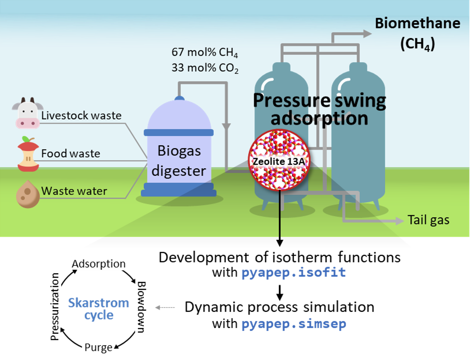
Figure. Schematic of bio-mathane production process.
Process description
Biogas produced through anaerobic digester is a gas that has a composition ratio of 67 and 33 mol% of CH4 and CO2 through a desulfurization pretreatment process. A two-component system real PSA simulation is performed based on process conditions to purify the biogas. The PSA process for biogas upgrading is adsorbed at 9 bar and desorbed at 1 bar, and the temperature and pressure of feed flow into 323 K. Here, we evaluate the commercial adsorbent, zeolite 13X for the biogas upgading.
Goal
The goal of this example is the simulation of biogas upgrading process with commercial adsorbent. Zeolite 13X and its pressure-uptake data could be found in the literature. This example contains isotherm fitting with given data(.csv), development of mixutre isotherm function and real PSA simulation.
Before we start, import pyAPEP packages. Also, users need to download adsorption data file (Example2_Zeolite13X.csv)
# pyAPEP package import
import pyadserver.isofit as isofit
import pyadserver.simsep as simsep

# Data treatment package import
import numpy as np
import pandas as pd

# Data visualization package import
import matplotlib.pyplot as plt
First, from the adsorption data samples, we need to find pure isotherm function for methane and carbon dioxide. Before developing isotherm, users need to define or import datasets. If the isotherm parameters already exist, users can use those parameters by defining isotherm function manually. Also, in this example, the single isotherm functions are used to simplify the process model.
# Data import
Data = pd.read_csv('Example2_Zeolite13X.csv')

# Pure isotherm definition
P_CO2 = Data['Pressure_CO2 (bar)'].dropna().values
q_CO2 = Data['Uptake_CO2 (mol/kg)'].dropna().values

P_CH4 = Data['Pressure_CH4 (bar)'].dropna().values
q_CH4 = Data['Uptake_CH4 (mol/kg)'].dropna().values

CO2_iso, _, _, _ = isofit.best_isomodel(P_CO2, q_CO2)
CH4_iso, _, _, _ = isofit.best_isomodel(P_CH4, q_CH4)
CO2_iso_ = lambda P,T: CO2_iso(P)
CH4_iso_ = lambda P,T: CH4_iso(P)

def MixIso(P, T):
   q1 = CO2_iso(P[0])
   q2 = CH4_iso(P[1])
   return q1, q2
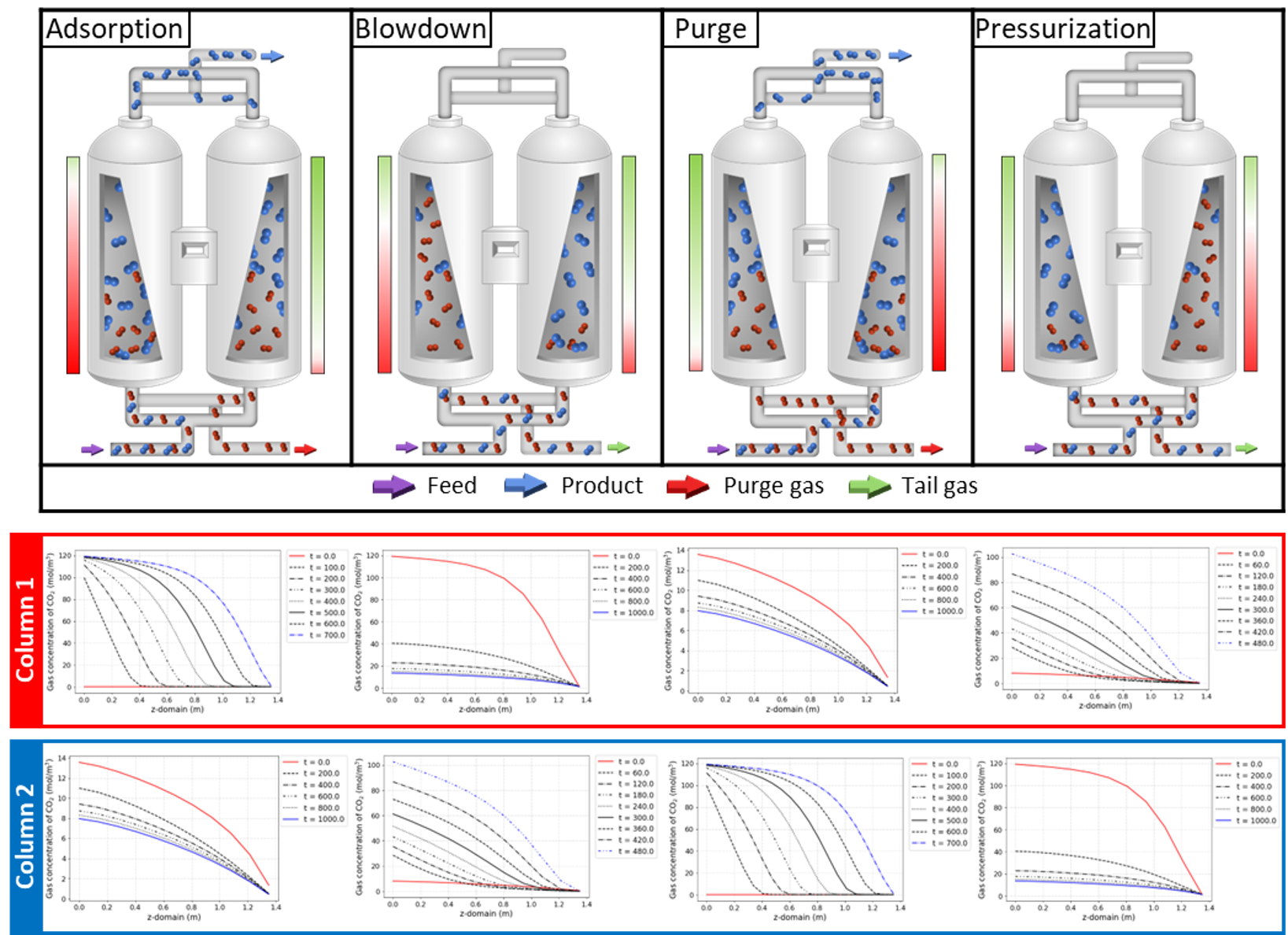
Next, we define and run an actual PSA process. A majority of the process parameters were the same as those in ref. In this example, Skarstrom cycle, which is the operation method for PSA process, is simulated in four stages of adsorption-blowdown-purge-pressurization.
# Column design
N = 21
L = 1.35
A_cros = np.pi*0.15**2
CR1 = simsep.column(L, A_cros, n_component=2, N_node = N)

### Sorbent prop
voidfrac = 0.37                  # (m^3/m^3)
D_particle = 12e-4               # (m)
rho = 1324                       # (kg/m^3)
CR1.adsorbent_info(MixIso, voidfrac, D_particle, rho)

### Gas prop
Mmol = [0.044, 0.016]            # (kg/mol)
mu_visco= [16.13E-6, 11.86E-6]   # (Pa s)
CR1.gas_prop_info(Mmol, mu_visco)

### Transfer prop
k_MTC  = [1E-2, 1E-2]            # (m/s)
a_surf = 1                       (m2/m3)
D_disp = [1E-2, 1E-2]            # (m^2/sec)
CR1.mass_trans_info(k_MTC, a_surf, D_disp)
dH_ads = [31.164e3,20.856e3]     # (J/mol)
Cp_s = 900
Cp_g = [38.236, 35.8]            # (J/mol/K)
h_heat = 100                     # (J/m2/K/s)
CR1.thermal_info(dH_ads, Cp_s, Cp_g, h_heat)
The operating and initial conditions are required to solve the differential equations. An appropriate value must be set for better convergence of the model. Each step of the Skarstrom cycle was implemented by adjusting the boundary and initial conditions. The parameter setting and simulation were repeated sequentially.
### Adsorption step ###
### Operating conditions
P_inlet = 9.5
P_outlet = 9
T_feed = 323
y_feed = [0.33,0.67]

Cv_inlet = 0.2E-1             # inlet valve constant (m/sec/bar)
Cv_outlet= 2.0E-1           # outlet valve constant (m/sec/bar)

Q_feed = 0.05*A_cros  # volumetric flowrate (m^3/sec)

CR1.boundaryC_info(P_outlet, P_inlet, T_feed, y_feed,
                  Cv_inlet, Cv_outlet,
                  Q_inlet = Q_feed,
                  assigned_v_option = True,
                  foward_flow_direction = True)

### Initial conditions
P_init = 9.25*np.ones(N)    # (bar)
y_init = [0.001*np.ones(N), 0.999*np.ones(N)] # (mol/mol)
T_init = T_feed*np.ones(N)
q_init = MixIso(P_init*np.array(y_init), T_init)

CR1.initialC_info(P_init, T_init, T_init, y_init, q_init)
print(CR1)
This example considers the mass, momentum, and energy balance equations, therefore run_mamoen function is used to run the simulation.
# Simulation run
y_res, z_res, t_res = CR1.run_mamoen(700,n_sec = 20,
                                 CPUtime_print = True)
Then, the adsorption step was simulated. The final results of this stage become the initial condition of the next step; the purge step and the boundary condition should be modified accordingly. After the simulation of the purge step, the blowdown step was implemented using the modified boundary condition and the final results of the previous step as an initial condition.
### Blowdown step ###
CR1.next_init()
CR1.change_init_node(11)

### Operating conditions
P_inlet = 9
P_outlet = 1
T_feed = 323
y_feed = [0.001,0.999]

Cv_inlet = 0E-1             # inlet valve constant (m/sec/bar)
Cv_outlet= 1E-1           # outlet valve constant (m/sec/bar)

CR1.boundaryC_info(P_outlet, P_inlet, T_feed, y_feed,
                  Cv_inlet, Cv_outlet,
                  foward_flow_direction = False)

y_res = CR1.run_mamoen(1000,n_sec = 10, CPUtime_print = True)
### Purge step ###
CR1.next_init()

### Operating conditions
P_inlet = 1.5
P_outlet = 1
T_feed = 323
y_feed = [0.001,0.999]

Cv_inlet = 1E-1             # inlet valve constant (m/sec/bar)
Cv_outlet= 4E-1           # outlet valve constant (m/sec/bar)

CR1.boundaryC_info(P_outlet, P_inlet, T_feed, y_feed,
                  Cv_inlet, Cv_outlet,
                  foward_flow_direction = False)

y_res = CR1.run_mamoen(1000,n_sec = 10, CPUtime_print = True)
To implement the final pressurization step, an iterative method is required in order to stabilize the simulation mainly because extreme pressure changes may result in calculation errors. The simulation was performed while repeatedly calculating a time of approximately 5 s, and the results of each iteration were stored to derive the final results for the pressurization step. Using iterative calculation, the column was pressurized from 1 bar to over 9 bar.
### Pressurization step ###
N = 11
R_gas = 8.3145      # 8.3145 J/mol/K

total_y = []
CR4 = copy.deepcopy(CR3)
CR4.next_init()
P_outlet = 1
P_inlet = 2
while P_outlet<9.1:
   ### Operating conditions
   T_feed = 323
   y_feed = [0.33,0.67]

   Cv_inlet =(P_inlet-P_outlet)*0.1             # inlet valve constant (m/sec/bar)
   Cv_outlet= 0E-1           # outlet valve constant (m/sec/bar)

   CR4.boundaryC_info(P_outlet, P_inlet, T_feed, y_feed,
                  Cv_inlet, Cv_outlet,
                  foward_flow_direction = True)
   y_res = CR4.run_mamoen(5,n_sec = 10,
                                    CPUtime_print = True)
   total_y.append(y_res)

   P = np.zeros(N)
   for ii in range(2):
      Tg_res = y_res[0][:,2*2*N : 2*2*N+N]
      P = P + y_res[0][:,(ii)*N:(ii+1)*N]*R_gas*Tg_res/1E5

   P_outlet = np.mean(P[-1])
   P_inlet = P_outlet+1.1
   # fig, ax = CR4.Graph_P(1, loc=[1.15,0.9])
   # plt.show()
   CR4.next_init()
The simulation results at each step are shown in below figure.
3. Development of machine learning-based model for PSA process
Background & Goal
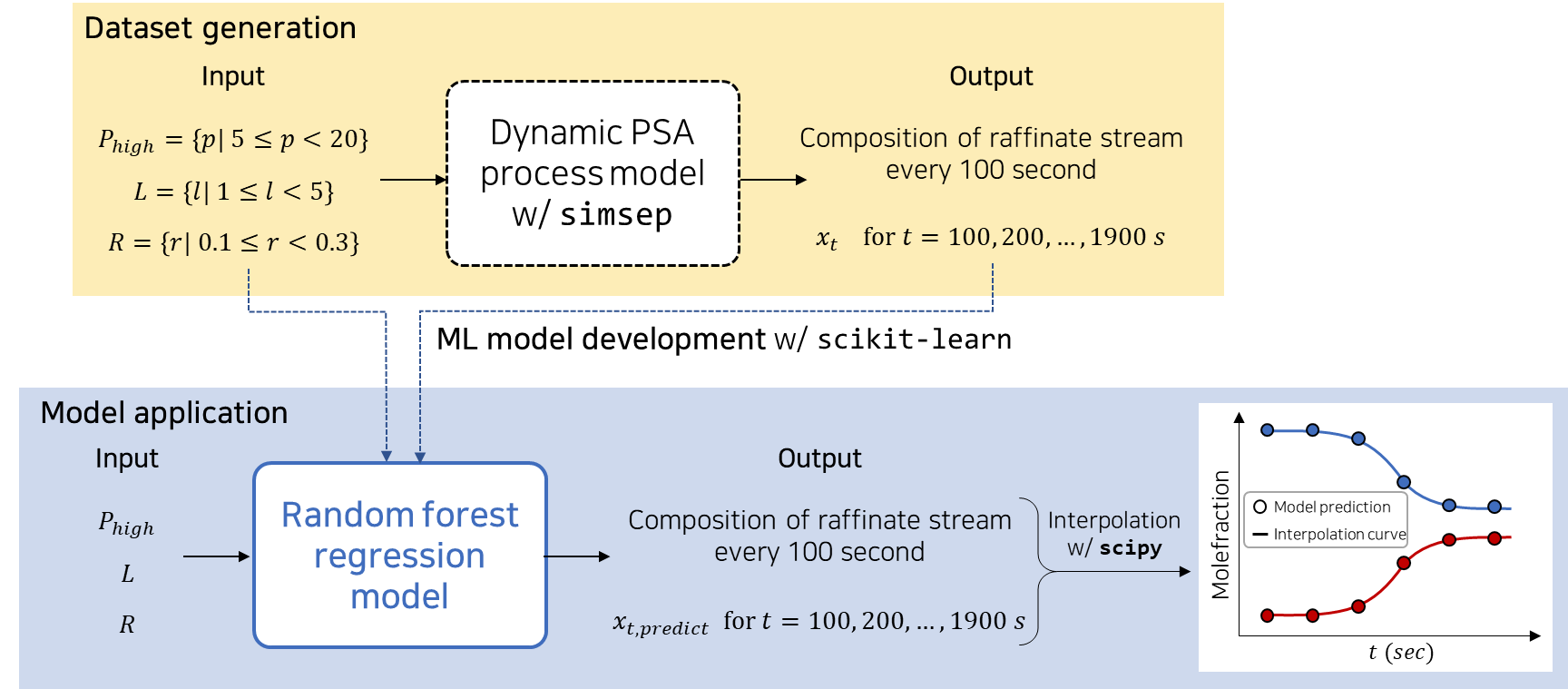
In previous section, a rigorous PSA process model for the separation of CO2 and CH4 was developed to derive the dynamic behavior of the process. Developed high-fidelity model is time-consuming for analysis according to various operating and design conditions. To resolve this issue, this case study developed a machine learning (ML) based PSA process model to predict the CO2 mole fraction of raffinate stream over time (t) and then estimate the breakthrough curve at each condition. This example consists of three steps: Dataset generation, model development, and application, as shown in figure below.
Before initiating this process, pyAPEP packages and other open-source Python packages were imported for data treatment and visualization. To develop a machine learning model for PSA process, scikit learn, and other analysis packages and modules are necessary. Additionally, the users are required to download an adsorption data file (Casestudy2_Zeolite13X.csv and Casestudy3_simsep_res.csv).
# pyAPEP package import
import pyapep.isofit as isofit
import pyapep.simsep as simsep

# Data treatment package import
import numpy as np
import pandas as pd

# Data visualization package import
import matplotlib.pyplot as plt

# ML model development and evaluation module import
from sklearn.model_selection import train_test_split
from sklearn.ensemble import RandomForestRegressor
from sklearn.metrics import r2_score

# Results anaysis module import
from itertools import product
from scipy.interpolate import interp1d
As in case study 2, isotherm is derived from :math:`CO_2` and :math:`CH_4` pressure-adsorption data using isofit modules. Then, for simplification, mixture isotherm is defined under the assumption that each component behaves independently.
# Data import, isotherm define
Data = pd.read_csv('Casestudy2_Zeolite13X.csv')

P_CO2 = Data['Pressure_CO2 (bar)'].dropna().values
q_CO2 = Data['Uptake_CO2 (mol/kg)'].dropna().values

P_CH4 = Data['Pressure_CH4 (bar)'].dropna().values
q_CH4 = Data['Uptake_CH4 (mol/kg)'].dropna().values

CO2_iso, CO2_p, CO2_name, CO2_err = isofit.best_isomodel(P_CO2, q_CO2)
CH4_iso, CH4_p, CO2_p, CH4_err = isofit.best_isomodel(P_CH4, q_CH4)
CO2_iso_ = lambda P,T: CO2_iso(P)
CH4_iso_ = lambda P,T: CH4_iso(P)

def MixIso(P, T):
   q1 = CO2_iso(P[0])
   q2 = CH4_iso(P[1])
   return q1, q2
Then, import simulation results and split the data into train and test dataset. The dataset was obtained by the dynamic simulation using simsep. A thousand repetitive calculations were performed by changing the length(L), radidus(R), and operating pressure (\(P_{high}\)) of the packing column, which affect the breakthrough time a lot. Each input variable was randomly set under domain range \(1 \le L \le 10\) (m), \(0.1 \le R \le 0.5\) (m) and \(5 \le P_{high} \le 20\) (bar). Output variables were set composition of raffinate stream at time t (100, 200, …, 1900 s).
# Random data import
data = pd.read_csv('Casestudy3_simsep_res.csv')

# Train-test split
x_var = ['L', 'R', 'P_high']
y_var = [f't{i}' for i in range(1, 20)]

data_x = data[x_var]
data_y = data[y_var]

x_train, x_test, y_train, y_test = train_test_split(data_x, data_y, test_size=0.3, shuffle= True, random_state = 102)
Using a machine learning library, scikit learn, PSA process model for the prediction of raffinate gas composition is developed using random forest regression algorithm. Because this example shows how to integrate pyAPEP with other Python packages, complex methods such as optimization of model structure and deep learning are not implemented. Based on compatibility with other packages shown in this example, users can apply the proposed package to various fields.
# Random forest regression model development and evaluation
model = RandomForestRegressor()
model.fit(x_train, y_train)

pred = model.predict(x_test)

plt.figure(dpi=200, figsize=(3*len(y_var),3))
for i in range(len(y_var)):
   plt.subplot(1, len(y_var), i+1)
   plt.scatter(y_test.iloc[:,i], pred[:,i], c='k', s = 1)
   r2 = r2_score(y_test.iloc[:,i], pred[:,i])
   plt.title(f'{(i+1)*100}s')
   plt.xlabel('Actual')
   plt.ylabel('Predict')
plt.tight_layout()
plt.show()
print('R2: ', r2)

# Model analysis in various conditions
L_dom = np.linspace(1, 5, 100)
P_dom = np.linspace(5, 20, 100)

LP_dom = np.array(list(product(L_dom, P_dom)))
x_dom = np.insert(LP_dom, 1, 0.25 ,axis= 1)

y_pred = model.predict(x_dom)
levels = np.linspace(0,y_pred.max(),100)

fig,ax=plt.subplots(1,len(y_var), figsize=(3*len(y_var),3), dpi=200)
for i in range(len(y_var)):
   y_dom = (y_pred[:,i]).reshape(100, 100)
   cp = ax[i].contourf(P_dom, L_dom, y_dom, cmap= 'Blues', levels=levels)
   ax[i].set_xlabel('Pressure (bar)')
   ax[i].set_ylabel('Length (m)')
fig.colorbar(cp, label=f'Molefraction (t={(i+1)*100}s)')
plt.tight_layout()
plt.show()

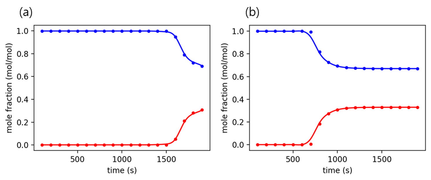
Using the developed machine learning model, the composition of the raffinate flow is predicted every 100 seconds, and a breakthrough curve is derived from the results. In the graph, the point is the composition predicted by the machine learning model, and the line is a function derived by interpolating each point.
# breakthrough curve prediction
for i in range(len(pred)):
   pred_tmp = pred[i,:]
   bt_crv = interp1d(np.arange(100, 2000, 100), pred_tmp, kind = 'cubic' )

   t_dom = np.arange(100, 1900)
   fn_pred = bt_crv(t_dom)

   if i%100 == 0:
      plt.figure(dpi=200, figsize=(4,3))
      plt.plot(t_dom, fn_pred, 'r',)
      plt.plot(t_dom, 1-fn_pred, 'b')
      plt.scatter(np.arange(100, 2000, 100), y_test.iloc[i,:],
                  s=10, c='r', label='Actual')
      plt.scatter(np.arange(100, 2000, 100), 1-y_test.iloc[i,:],
                  s=10, c='b', label='Actual')
      plt.xlabel('time (s)')
      plt.ylabel('mole fraction (mol/mol)')
      plt.tight_layout()
      plt.show()
