Example 1: Numerous membrane screening

Example description

In the first example, a comprehensive membrane process simulation was conducted to assess numerous Metal-Organic Framework (MOF) membranes at the process scale. Typically, the evaluation of MOF membranes relies on high-throughput screening, which considers membrane properties such as diffusion selectivity and membrane selectivity. However, the performance of membrane separation processes is significantly influenced by both the membrane properties and process operation conditions. To accurately evaluate a membrane, conducting a process simulation for each material is crucial. In this example, pySembrane was used to identify potential MOFs within the CoRE MOF database, as depicted in Fig. 1 (a). The procedure began with molecular simulations for MOFs in the CoRE MOF database to obtain membrane properties. Subsequently, permeance, which is an essential parameter for process simulation, was derived using the membrane property calculation module. Membrane process simulation was then conducted for each MOF. The process simulation module derives the hydrogen (H₂) purity on each side, considering both the retentate and permeate outlets. MOFs that failed to produce H₂ with purity exceeding 99.9% on both sides were determined to be unsuitable for H₂ separation and were eliminated. Conversely, MOFs exhibiting high-purity hydrogen on either side were selected as potential candidates, warranting further in-depth analyses. Additional details regarding the parameters for the database, molecular simulation, and process simulation used in this example are provided in following section.

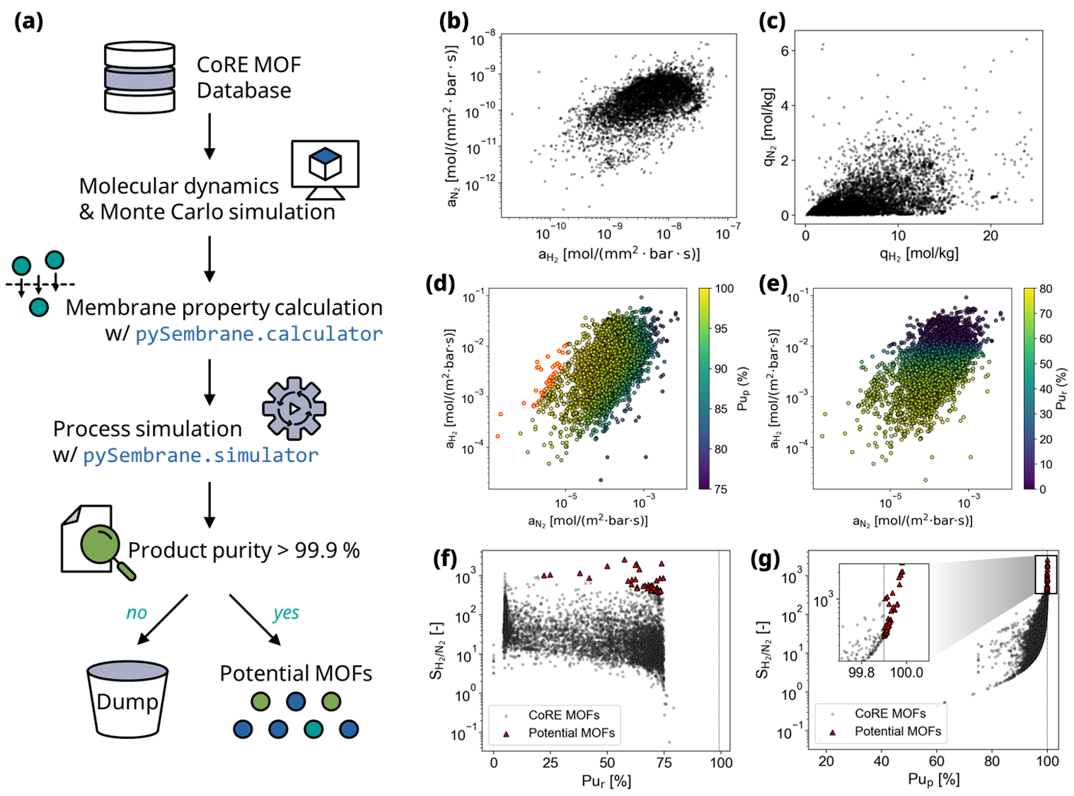
Casestudy1 — **Fig. 1** Workflows and results of example 1. (a) MOF membrane evaluation method using pySembrane by applying to CoRE MOF 2019 database. Scatter plots of (b) permeance and (c) gas uptake for H₂ and N₂, obtained from the membrane property module and molecular simulation, respectively. Permeance scatter plots colored according to H₂ purity for (d) permeate and (e) retentate sides, with MOFs identified as potential membranes for their high product purity highlighted in red. Results of comparative analysis between H₂ purity and conventional evaluation metric, selectivity (\(S_{H_2/N_2}\)) for (f) permeate and (g) retentate side, respectively. Each scatter plot includes 6,086 MOFs, which are pre-screened based on structural properties.

Method

To evaluate the MOFs selected from pre-screening based on process performance, it is necessary to determine membrane properties. In this study, gas uptake and self-diffusivity were derived through Grand Canonical Monte Carlo simulation (GCMC) and molecular dynamics simulation (MD). Subsequently, membrane property, gas permeance, is derived using the property calculator module. Firstly, GCMC and MD simulations were performed using the RASPA simulation software. Adsorption of gases was examined for single-component H₂ and N₂ at 6 bar and 2 bar, respectively. Intermolecular interactions were defined using the Lennard−Jones (LJ) potential, and the Lorentz−Berthelot mixing rule was applied to parametrize the effective pair potentials. The LJ parameters of the framework atoms were obtained using the DREIDING and UFF force fields. The CoRE MOF database provides DDEC partial charges of each MOF, and the potential parameters are determined from these two classic force fields. N₂ and H₂ were modeled as three-site rigid molecules, where partial atomic charges were placed on two real atoms and dummy atoms were introduced to the center of mass to maintain charge neutrality. The interactions between non-identical atoms were estimated using Lorentz-Berthelot mixing rules. Although the Feynman-Hibbs effect is often used to account for quantum mechanical effects significant at cryogenic temperatures, this study assumed classical molecular behavior due to the operational temperature at 313.13 K. The cut-off radius for the LJ interactions was set as 12.5 Å by the literature. In our previous study, we validated the method through a comparison between simulation results and experimental results from the literature. MD simulations were conducted to determine the self-diffusivity (\(\mathcal{D}\)) of both H₂ and N₂. For each gas component, simulations were performed with thirty molecules at infinite dilution. The simulation procedure included 1,000 initialization cycles, followed by 10,000 production cycles, totaling 1,000,000 cycles. The simulations were executed in the NVT ensemble with a time step of 0.5 fs. Self-diffusivity was calculated from the MD simulation results using the CropMSD and CalculSelfDiff functions within the property calculation module.

Using the membrane property, a membrane process model is developed for each MOF material with process parameters as listed in Table 1. After the process simulation ended, the product purity at the outlet of each stream is calculated with the following equation:

\[Pu_{k,i} = \frac{F_{k,i}}{\sum_{i}F_{k,i}} \times 100(\%) \ \ \mathrm{for} \ k= f \ \mathrm{or} \ p\]

where \(Pu_{k,i}\) and \(F_{k,i}\) refers to the purity and flow rate of component \(i\) in \(k\) stream, which is feed (\(f\)) or permeate (\(p\)) side. If the purity of the product does not exceed the standard 99.9% on any side, those MOFs are excluded, and if this constraint is met, further analysis is performed in the second example. In this example, 47 out of 6,086 MOFs were selected as potential MOFs.

**Table 1** Membrane process parameters.
Parameters	Value
Temperature (T) [K]	273
Feed pressure (P_f) [bar]	20
Permeate pressure (P_p) [bar]	1
Feed flow (F_f) [mol/s]	0.7
Feed H₂ composition (y_f) [mol%]	75
Feed N₂ composition (y_f) [mol%]	25
Module diameter (d_m) [m]	0.3
Fiber inner diameter (d_i) [mm]	10
Fiber outer diameter (d_o) [mm]	25
Fiber length (L) [m]	0.6
Number of fibers (N_f)	100
Module configuration	COFS
Sweep gas	No

Results analysis

Fig. 1 (b) shows the permeance of N₂ and H₂ obtained from the property calculation module. Generally, the permeance of H₂ is higher than that of N₂, as demonstrated in (c), where H₂ exhibits a larger gas uptake than N₂.

Fig. 1 (d) and (e) present the H₂ purity on the permeate and retentate sides, respectively, after the process simulation of each MOF membrane. The purity of H₂ on the permeate side is higher than that on the retentate side. Furthermore, the gas permeance, which influences the purity of each side, differs. On the permeate side, the purity tends to increase as N₂ permeance decreases relative to H₂ permeance. This phenomenon is attributed to the variance in the amount of nitrogen permeating from the retentate side to the permeate side based on the nitrogen permeance. Conversely, on the retentate side, the H₂ purity tends to increase as the H₂ permeance decreases relative to N₂. This phenomenon results from the difference in the amount of H₂ permeated from the retentate side. In essence, membrane performance in the process is affected by not only the absolute permeance value of each gas but also the relative permeance and the process conditions. As a result of the process simulation, 47 MOFs exhibiting a purity of 99.9 % or higher, surpassing the threshold, were selected, and these potential MOFs are highlighted with a red border.

Fig. 1 (f) and (g) show the correlation between H₂ purity and membrane selectivity on each side. As shown in the figures, the membrane selectivity and product purity are not proportional, which shows that the existing simple evaluation index, selectivity, cannot represent the performance in the actual process. For example, a MOF with the highest selectivity cannot be selected as a potential MOF because it cannot produce high-purity hydrogen on any side. If the material was evaluated using only selectivity, the majority of MOFs shown in red would not be selected as potential MOFs, which poses the risk of making a large error. Therefore, evaluation from a process perspective must be accompanied by a membrane evaluation.

Source code

Initially, the required Python libraries are imported. The pySembrane library is utilized for deriving membrane properties and conducting membrane process simulation models, while the numpy, matplotlib, and pandas packages are employed for data processing, visualization, and handling Excel data, respectively. Additionally, the data used in the example is imported, encompassing self-diffusivity, gas uptake, and density data for pre-screened MOFs.

from simulator import *
from calculator import *

import numpy as np
import matplotlib.pyplot as plt
import pandas as pd

data = pd.read_csv('240219_Casestudy1_data_rev.csv', index_col=0)

A ‘for’ loop is executed to derive the membrane properties of 6,086 MOF materials. In each iteration, the density of each MOF, as well as the partial pressures of H₂ and N₂, gas uptake, and self-diffusivity, are loaded. The CalculPermeance function is then utilized to derive permeance and permeability, with the results being recorded.

D_inner = 100*1e-1            # Membrane inner diameter (mm)
D_outer = 250*1e-1            # Membrane outer diameter (mm)
thickness = (D_outer-D_inner)/2

q_list = []
a_i = []
p_i = []
for ii in range(len(data)):
    target_mof = data.iloc[ii,:]
    pp_H2, DD_H2,qq_H2  = target_mof[['P_H2(bar)', 'D_H2(m^2/s)','q_H2(mol/kg)']].values
    pp_N2, DD_N2,qq_N2  = target_mof[['P_N2(bar)', 'D_N2(m^2/s)','q_N2(mol/kg)']].values
    rho = target_mof['Density(kg ads/m^3)']

    a_H2 = CalculPermeance(pp_H2, DD_H2*1e6, qq_H2, rho*1e-9, thickness)
    a_N2 = CalculPermeance(pp_N2, DD_N2*1e6, qq_N2, rho*1e-9, thickness)

    a_i.append([a_H2, a_N2])
    p_i.append([a_H2*thickness/(3.4e-14), a_N2*thickness/(3.4e-14)])        # Permeability (Barrer)

data[['a_H2(mol/(mm^2 bar s))', 'a_N2(mol/(mm^2 bar s))']] = np.array(a_i)
data[['P_H2(Barrer)', 'P_N2(Barrer)']] = np.array(p_i)

The code provided below is designed to plot Fig. 1 (b) and (c), showcasing the distribution of gas uptake and permeance for hydrogen and nitrogen gases, respectively.

plt.figure(dpi=90, figsize=(5,4))
plt.scatter(data['a_H2(mol/(mm^2 bar s))'], data['a_N2(mol/(mm^2 bar s))'],
            c='k', alpha=0.3, s=5)
plt.ylabel('a$_{\mathrm{N_2}}$ [$\mathrm{mol/(mm^2\cdot bar\cdot s)}$]')
plt.xlabel('a$_{\mathrm{H_2}}$ [$\mathrm{mol/(mm^2\cdot bar\cdot s)}$]')
plt.yscale('log')
plt.xscale('log')
plt.show()

plt.figure(dpi=90, figsize=(5,4))
plt.scatter(data['q_H2(mol/kg)'], data['q_N2(mol/kg)'],
            c='k', alpha=0.3, s=5)
plt.ylabel('q$_{\mathrm{N_2}}$ [mol/kg]')
plt.xlabel('q$_{\mathrm{H_2}}$ [mol/kg]')
plt.show()

Parameters necessary for the membrane separation process simulation are defined. The parameters set in the following code are uniformly applied across all developed process models.

### Module design ###
n_component = 2               # number of gas components
config = 'COFS'               # module configuration
L = 0.6*1e3                   # fiber length (mm)
D_module = 0.3*1e3            # Module diameter (mm)
N_fiber = 100                 # number of fiber (-)
N = 100                       # number of nodes (-)

### Membrane information ###
D_inner = 100*1e-1            # Membrane inner diameter (mm)
D_outer = 250*1e-1            # Membrane outer diameter (mm)

### Gas property ###
Mw_i = np.array([2e-3, 28e-3])                 # molar weight (kg/mol)
rho_i = np.array([0.08988, 1.1606])*1e-9       # density (kg/mm3)
mu_i = np.array([0.94e-3, 1.89e-3])            # viscosity (Pa s)

### Mass transfer property ###
k_mass = 1e-1              # Mass transfer coeff. (mm/s)

### Operating conditions ###
# Boundary conditions
P_feed = 20                         # pressure of feed side (bar)
T = 273                             # temperature (K)
F_feed = 0.7                        # feed flow rate (mol/s)
y_feed = np.array([0.75, 0.25])     # mole fraction (H2, N2)

A loop is employed to develop a membrane process model for each MOF and to save the outcomes. The membrane properties derived for each MOF are specified, and the membrane process model is defined. Following the simulation, the purity of the product is calculated by utilizing the flow rates at the stream outlet (F_perm and F_ret). A post-treatment of the simulation results is performed using a mass balance equation to ensure the flow rates are always positive. The purity derived on the retentate and permeate sides for each MOF is then saved in a .csv file. The saved results can be downloaded from GitHub.

### Membrane process simulation ###
pu_list = []
for ii in range(len(data)):
    target_mof = data.iloc[ii,:]
    a_perm = np.array([target_mof[ii] for ii in ['a_H2(mol/(mm^2 bar s))', 'a_N2(mol/(mm^2 bar s))']])
    mem = MembraneProc(config, L, D_module, N_fiber,
                n_component, n_node = N)
    mem.membrane_info(a_perm, D_inner, D_outer)
    mem.gas_prop_info(Mw_i, mu_i, rho_i)
    mem.mass_trans_info(k_mass)
    mem.boundaryC_info(y_feed, P_feed, F_feed, T)
    mem.initialC_info()

    res = mem.run_mem(cp=False, cp_cond = [1, 298])
    err = mem.MassBalance()

    F_perm = res[-1, n_component:n_component*2]
    F_ret = res[-1, :n_component]
    F_perm[F_ret<0] = (F_feed*y_feed)[F_ret<0]
    F_ret[F_ret<0] = 0

    pu_ = [flow[0]/sum(flow) if sum(flow)>0 else 0 for flow in [F_ret, F_perm]]
    pu_list.append(pu_)
data[[f'Pu_ret_{F_feed}', f'Pu_perm_{F_feed}']] = np.array(pu_list)
data.to_csv('240219_Casestudy1_results.csv')

Below is the code for visualizing the simulation results, which upon execution, yields Fig. 1 (g–d). Consequently, this example facilitates the selection of 47 MOFs that exceed a hydrogen purity of 99.9 %.

### Results plots ###
ex1_res = pd.read_csv('240219_Casestudy1_results.csv')
pot_MOF = ex1_res[(ex1_res[f'Pu_ret_{F_feed}'] > 0.999) |(ex1_res[f'Pu_perm_{F_feed}'] > 0.999)]

plt.figure(dpi=90, figsize=(6,5))
plt.scatter(ex1_res['a_N2(mol/(mm^2 bar s))']*1e6, ex1_res['a_H2(mol/(mm^2 bar s))']*1e6,
            c=ex1_res[f'Pu_perm_{F_feed}']*100,
            edgecolors=['k' if targ<=0.999 else 'r' for targ in ex1_res[f'Pu_perm_{F_feed}']],
            alpha=[0.7 if targ<=0.999 else 1 for targ in ex1_res[f'Pu_perm_{F_feed}']],
            s=20,vmin=75, vmax=100
            )
plt.colorbar(label='Pu$_{\mathrm{p}}$ (%)')
plt.ylabel('a$_{\mathrm{H_2}}$ [$\mathrm{mol/(m^{2}·bar·s)}$]')
plt.xlabel('a$_{\mathrm{N_2}}$ [$\mathrm{mol/(m^{2}·bar·s)}$]')
plt.yscale('log')
plt.xscale('log')
plt.show()

plt.figure(dpi=90, figsize=(6,5))
plt.scatter(ex1_res['a_N2(mol/(mm^2 bar s))']*1e6, ex1_res['a_H2(mol/(mm^2 bar s))']*1e6,
            c=ex1_res[f'Pu_ret_{F_feed}']*100,
            edgecolors=['k' if targ<=0.999 else 'r' for targ in ex1_res[f'Pu_ret_{F_feed}']],
            alpha=[0.7 if targ<=0.999 else 1 for targ in ex1_res[f'Pu_ret_{F_feed}']],
            s=20,
            vmin=0, vmax=80
            )
plt.colorbar(label='Pu$_{\mathrm{r}}$ (%)')
plt.ylabel('a$_{\mathrm{H_2}}$ [$\mathrm{mol/(m^{2}·bar·s)}$]')
plt.xlabel('a$_{\mathrm{N_2}}$ [$\mathrm{mol/(m^{2}·bar·s)}$]')
plt.yscale('log')
plt.xscale('log')
plt.show()

ex1_res['S_H/N'] = ex1_res['a_H2(mol/(mm^2 bar s))']/ex1_res['a_N2(mol/(mm^2 bar s))']
pu_max = (ex1_res[['Pu_ret_0.7', 'Pu_perm_0.7']]).max(axis=1)

plt.figure(dpi=90, figsize=(5,4))
plt.scatter(ex1_res['Pu_ret_0.7'][pu_max<=0.999]*100, ex1_res['S_H/N'][pu_max<=0.999],
            c='grey', alpha=0.3, edgecolors='k',
            s = 5, label='CoRE MOFs',)
plt.scatter(ex1_res['Pu_ret_0.7'][pu_max>0.999]*100, ex1_res['S_H/N'][pu_max>0.999],
            c='r', alpha=1, s=30,
            edgecolors='k', label='Potential MOFs',
            marker='^')
plt.axvline(99.9, c='k', linestyle='--', linewidth = 0.5)
plt.legend(fontsize=14)
plt.xlabel('Pu$\mathrm{_{r}}$ [%]')
plt.ylabel('S$\mathrm{_{H_2/N_2}}$ [-]')
plt.yscale('log')
plt.tight_layout()
plt.show()

plt.figure(dpi=90, figsize=(5,4))
plt.scatter(ex1_res['Pu_perm_0.7'][pu_max<=0.999]*100, ex1_res['S_H/N'][pu_max<=0.999],
            c='grey', alpha=0.3, edgecolors='k',
            s = 5, label='CoRE MOFs',)
plt.scatter(ex1_res['Pu_perm_0.7'][pu_max>0.999]*100, ex1_res['S_H/N'][pu_max>0.999],
            c='r', alpha=1, s=30,
            edgecolors='k', label='Potential MOFs',
            marker='^')
plt.axvline(99.9, c='k', linestyle='--', linewidth = 0.5)
plt.xlabel('Pu$\mathrm{_{p}}$ [%]')
plt.ylabel('S$\mathrm{_{H_2/N_2}}$ [-]')
plt.yscale('log')
plt.legend(fontsize=14, loc='lower left')
plt.tight_layout()
plt.show()