Example 3: Integrated process simulations with other processes for process level evaluation

Example description

In the last example, the process model is developed including the green NH₃ decomposition and H₂ purification, and the plant scale analysis is conducted for the selected optimal MOF membrane, integrating with the membrane process module. As shown in Fig. 1 (a), the processes, excluding the membrane process module, were developed using commercial software, Aspen Plus, while the membrane process module was modeled using the pySembrane. The integration between the two software tools took place in the Python environment, and each process model exchanged stream flow and pressure results to perform simulations. Fig. 1 (b) illustrates the integrated process, and each software is highlighted in blue and green, respectively. The entire process involves the decomposition of transported green NH₃ in the reactor, separation of unreacted NH₃ in the pressure swing adsorption process (PSA1), and hydrogen production in the PSA2 unit. The stream produced at the bottom of PSA2 contains a significant amount of hydrogen, necessitating additional separation processes to increase the H₂ production. Using pySembrane, the outlet stream of the compressor unit (Comp) is set as the feed for membrane process simulation, and the results are then utilized as input variables in Aspen Plus to determine the total production rate of H₂.

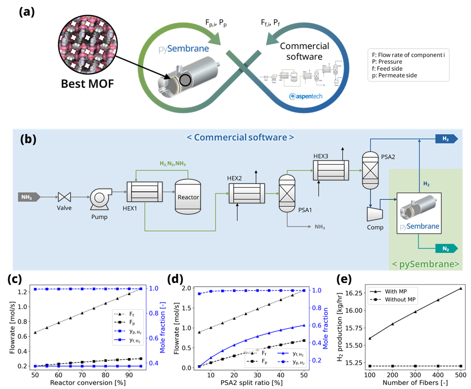
Casestudy3 — **Fig. 1** (a) Schematic of the integration between pySembrane and commercial software in example 3. (b) green ammonia decomposition and hydrogen production process model using both commercial software and pySembrane. Flow rate and mole fraction results for each stream corresponding to the process variables: (c) NH₃ conversion of the reactor and (d) split ratio of PSA2 unit. (e) Comparison study of H₂ production rate between with and without membrane process according to fiber length of membrane process module.

Plant model devlopment

The plant model developed by commercial software and the membrane separation model developed by pySembrane are integrated. Fig. 2 shows the entire process of decomposing green NH₃ and producing green H₂ by separating H₂ and N₂. The process model was simulated using Aspen Plus V14.0 with the Peng-Robinson fluid package for the thermodynamic model. Stream 101, the green NH₃ feedstock, is first decompressed via a valve (VLV-100) and subsequently pressurized to 8.5 bar using a pump (P-100). This feed stream is then heated to 100 \(^{\circ} C\) in the heat exchanger (HX-101) before entering the NH₃ decomposition reactor (R-200). Through the reactor, green NH₃ is converted to H₂ and N₂, and a high-temperature H₂/N₂ mixture stream containing unreacted NH₃ is used as a hot stream of the heat exchanger (HX-100) for feed heating, which is then cooled to 105 \(^{\circ} C\). The reactor outlet stream repeats the cooling and separation process to produce the final product, H₂. Initially, unreacted NH₃ is removed in the pressure swing adsorption process (ADS-300) after cooling to 40 \(^{\circ} C\) in a heat exchanger (HX-102) using cooling water. The H₂/N₂ mixture gas produced by the raffinate flow of the PSA process goes through the second PSA process (PSA-400) to produce high-purity H₂. Since the tail gas produced in PSA-400 still contains a large amount of H₂, additional H₂ is produced through the membrane-based separation process after being pressurized by a compressor (COMP-100) to increase production. Table 1 lists the detailed specifications of each unit and feed stream.

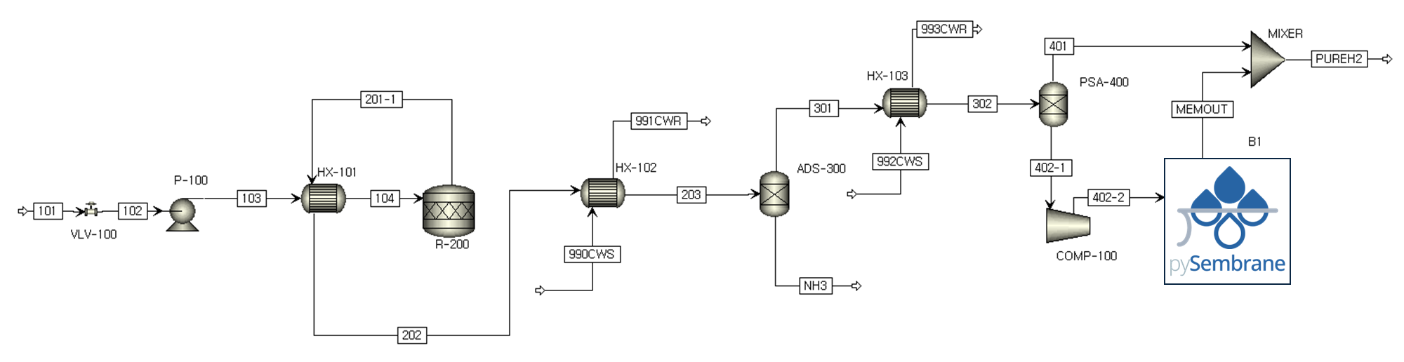
Casestudy3ProcessModel — **Fig. 2** Process diagram of green ammonia cracking and hydrogen production system.

**Table 1** Specification of each model and feed stream.
Model	Specification
VLV-100	Adiabatic flash
VLV-100	Pressure: 6bar
P-100	Pressure increase: 250kPa
P-100	Pump efficiency: 75%
HX-101	Cold stream outlet temperature: 100 \(^{\circ} C\)
R-200	Reaction: 2NH₃->3H_2`+N:sub:`2
	Temperature: 600:math:^{circ} C
	Fraction of conversion:0.9
	Pressure: 8.5bar
HX-102	Cooling water inlet temperature: 15 \(^{\circ} C\)
HX-102	Hot stream outlet temperature: 40 \(^{\circ} C\)
ADS-300	Split fraction of H₂,N₂,O₂ and H₂ O: 1
HX-103	Cooling water inlet temperature: 15 \(^{\circ} C\)
HX-103	Hot stream outlet temperature: 40 \(^{\circ} C\)
PSA-400	Split fraction of H₂: 0.8
COMP-100	Pressure: 11.15bar
COMP-100	Compressor efficiency: 0.75

Results analysis

Fig. 1 (c–d) presents the simulation results corresponding to the conversion rate of the NH₃ decomposition reactor and the ratio split to the bottom in the PSA2 unit. \(F_f\) and \(y_f\) represent the flow rate and composition of the feed entering the membrane module, respectively, and \(F_p\) and \(y_p\) denote the flow rate and composition of the permeate side produced in the membrane process. As shown in Fig. 1 (c), with an increase in the conversion rate of the NH₃ decomposition reactor, the flow rates of N₂ and H₂ increase, leading to an increase in the feed flow rate of the module. Consequently, flow rates and H₂ purity on the permeate side increased. Fig. 1 (d) illustrates the PSA2 split ratio, which represents the ratio of the flow rate entering the membrane process to the total flow rate produced in the PSA2 unit, as it increases, indicating an increase in both the feed flow rate and composition. As a result, the H₂ production on the permeate side is increased, with the purity of H₂ showing a tendency to increase significantly. Fig. 1 (e) compares the total production of H₂ according to the number of fibers in the membrane process module, depending on the presence of the membrane process (MP). Without a membrane process, the production rate is low at 15.2 kg/hr, but with additional H₂ production from the stream discarded by the membrane process, the overall production of H₂ significantly increases. Moreover, as the number of fibers in the module increases, the H₂ production rate increases significantly, contributing to the overall productivity of the process. This example allows for the analysis of the impact of operating conditions in upstream processes on the membrane process and the influence of membrane process conditions on the overall process.

Source code

First, import the necessary libraries required to solve the example. Then, run Aspen Plus to open the example file and define each stream and unit block.

### Load process model ###
import os
import win32com.client as win32
import numpy as np
import matplotlib.pyplot as plt
import pandas as pd
from simulator import *

filename = 'Casestudy/GreenNH3.apw'
sim = win32.Dispatch("Apwn.Document")
sim.InitFromArchive2(os.path.abspath(filename))
sim.Visible = True

MyBlocks = sim.Tree.Elements("Data").Elements("Blocks")
MyStreams = sim.Tree. Elements("Data").Elements("Streams")

ProcOut = MyStreams.Elements("402-2").Elements("Output")

Define the parameters needed for the membrane process simulation. However, the operating conditions of membrane process are determined by the results of stream 402-2 within the Aspen Plus model, so these results are imported.

### Module design ###
n_component = 2               # number of gas components
config = 'COFS'               # module configuration
L = 0.6*1e3                   # fiber length (mm)
D_module = 0.3*1e3            # Module diameter (mm)
N_fiber = 100                 # number of fiber (-)
N = 100                       # number of nodes (-)

### Membrane property ###
D_inner = 100*1e-1            # Membrane inner diameter (mm)
D_outer = 250*1e-1            # Membrane outer diameter (mm)

### Gas property ###
Mw_i = np.array([2e-3, 28e-3])                 # molar weight (kg/mol)
rho_i = np.array([0.08988, 1.1606])*1e-9       # density (kg/mm3)
mu_i = np.array([0.94e-3, 1.89e-3])            # viscosity (Pa s)

### Mass transfer property ###
k_mass = 1e-1              # Mass transfer coeff. (mm/s)

# Load Asepn results (Operating conditions)
P_feed = ProcOut.Elements("PRES_OUT").Elements("MIXED").Value  # pressure of feed side (bar)
T = ProcOut.Elements("RES_TEMP").Value + 273.15
F_feed = ProcOut.Elements("RES_MOLEFLOW").Value/60/60*1e3
x_H2 = ProcOut.Elements("MOLEFRAC").Elements("MIXED").Elements("HYDRO-01").Value
x_N2 = ProcOut.Elements("MOLEFRAC").Elements("MIXED").Elements("NITRO-01").Value
y_feed = np.array([x_H2, x_N2])     # mole fraction (H2, N2)

Load the membrane properties of the best MOF determined from a previous example from an Excel file, and then conduct the membrane process simulation.

data = pd.read_csv('240221_Casestudy2_results.csv')
best_mof = data.sort_values(by='LCOH_opt').iloc[0,:]
a_H2, a_N2 = best_mof[['a_H2(mol/(mm^2 bar s))', 'a_N2(mol/(mm^2 bar s))']]
a_perm = np.array([a_H2, a_N2])

mem = MembraneProc(config, L, D_module, N_fiber,
            n_component, n_node = N)
mem.membrane_info(a_perm, D_inner, D_outer)
mem.gas_prop_info(Mw_i, mu_i, rho_i)
mem.mass_trans_info(k_mass)
mem.boundaryC_info(y_feed, P_feed, F_feed, T)
mem.initialC_info()

res = mem.run_mem(cp=False, cp_cond = [1, 298])
err = mem.MassBalance()
mem.PlotResults()

Utilize the results of the membrane process simulation as input for the MEMOUT stream in the plant model. Enter the flow rate for each component, temperature, and pressure, then run the Aspen Plus file. This calculates the additional H₂ production through the membrane module to derive the total H₂ production.

### Process integration ###
MemOut = MyStreams.Elements("MEMOUT").Elements("Input")
MemOut.Elements("FLOW").Elements("MIXED").Elements("HYDRO-01").Value = res[-1,2]*60*60*1e-3
MemOut.Elements("FLOW").Elements("MIXED").Elements("NITRO-01").Value = res[-1,3]*60*60*1e-3
MemOut.Elements("TEMP").Elements("MIXED").Value = T
MemOut.Elements("PRES").Elements("MIXED").Value = res[-1,-1]

sim.Run2()
sim.Save()

PureH2 = MyStreams.Elements("PUREH2").ElementS("Output").ElementS("RES_MASSFLOW").Value
print("Total H2 production: ", PureH2, "kg/hr")

Perform sensitivity analysis to analyze the impact of various process variables. Below, a loop repeatedly simulates the process models as the NH3 conversion rate in the NH₃ decomposition reactor (R-200) changes from 50 to 95%.

### Sensitivity analysis ###
## Sensitivity analysis
conv_list = np.linspace(0.5, 0.95, 10)
H2_prod = []
for _conv in conv_list:
    Rxr = MyBlocks.Elements("R-200").Elements("Input").Elements("CONV").Elements("1")
    Rxr.Value = _conv

    sim.Run2()
    sim.Save()

    # Operating conditions
    P_feed = ProcOut.Elements("PRES_OUT").Elements("MIXED").Value  # pressure of feed side (bar)
    T = ProcOut.Elements("RES_TEMP").Value + 273.15
    F_feed = ProcOut.Elements("RES_MOLEFLOW").Value/60/60*1e3
    x_H2 = ProcOut.Elements("MOLEFRAC").Elements("MIXED").Elements("HYDRO-01").Value
    x_N2 = ProcOut.Elements("MOLEFRAC").Elements("MIXED").Elements("NITRO-01").Value
    y_feed = np.array([x_H2, x_N2])     # mole fraction (H2, N2)
    Ff_z0_init = list(y_feed*F_feed)

    mem.boundaryC_info(y_feed, P_feed, F_feed, T)
    mem.initialC_info()

    res = mem.run_mem(cp=False, cp_cond = [1, 298])
    err = mem.MassBalance()

    MemOut = MyStreams.Elements("MEMOUT").Elements("Input")
    MemOut.Elements("FLOW").Elements("MIXED").Elements("HYDRO-01").Value = res[-1,2]*60*60*1e-3
    MemOut.Elements("FLOW").Elements("MIXED").Elements("NITRO-01").Value = res[-1,3]*60*60*1e-3
    MemOut.Elements("TEMP").Elements("MIXED").Value = T-273.15
    MemOut.Elements("PRES").Elements("MIXED").Value = res[-1,-1]

    sim.Run2()
    sim.Save()

    PureH2 = MyStreams.Elements("PUREH2").ElementS("Output").ElementS("RES_MASSFLOW").Value
    H2_prod.append([F_feed, x_H2, x_N2, res[-1,0], res[-1,1], res[-1,2], res[-1,3], PureH2])

Below is the code to plot the flow rate and composition of the feed entering the membrane module and the flow rate and composition of the permeate side produced as reactor conversion changes, yielding Fig. 1 (c) upon execution.

### Results plot ###
conv_nd = np.array(H2_prod)

fig, ax1= plt.subplots(dpi=200, figsize=(6,4))
line2 = ax1.plot(np.array(conv_list)*100, conv_nd[:,0], marker='^', c='k',
        label='F$\mathrm{_{f}}$', linestyle=':')
line7 = ax1.plot(np.array(conv_list)*100, conv_nd[:,5], marker='s', c='k',
        label='F$\mathrm{_{p}}$', linestyle='--')
ax1.set_ylabel('Flowrate [mol/s]')
ax2 = ax1.twinx()
line8 = ax2.plot(np.array(conv_list)*100,
                conv_nd[:,1],
                marker='s', c='b',
                label='y$\mathrm{_{f,H_2}}$', linestyle='-')
line6 = ax2.plot(np.array(conv_list)*100,
                conv_nd[:,5]/conv_nd[:,5:7].sum(axis=1),
                marker='s', c='b',
                label='y$\mathrm{_{p,H_2}}$', linestyle='--')
ax2.set_ylabel('Mole fraction [-]')
ax2.yaxis.label.set_color('b')
ax2.spines["right"].set_edgecolor('b')
ax2.tick_params(axis='y', colors='b')

plots = line2+line7+ line6+line8
labels = [l.get_label() for l in plots]
ax1.legend(plots, labels, loc='center right', fontsize=14)
ax1.set_xlabel('Reactor conversion [%]')
plt.tight_layout()
plt.show()

Below is the code for comparing the process performance as the split ratio of the stream produced in the second PSA process (PSA-400), specifically stream 402-1, changes from 50 to 95%. The split ratio is adjusted and the simulation is repeated through a loop, with the results being saved.

## Sensitivity analysis
split_list = np.linspace(0.5, 0.95, 10)
split_res = []
for _split in split_list:

    Rxr = MyBlocks.Elements("PSA-400").Elements("Input").Elements("FRACS").Elements("401").Elements("MIXED").Elements("HYDRO-01")
    Rxr.Value = _split

    sim.Run2()
    sim.Save()

    # Operating conditions
    P_feed = ProcOut.Elements("PRES_OUT").Elements("MIXED").Value  # pressure of feed side (bar)
    T = ProcOut.Elements("RES_TEMP").Value + 273.15
    F_feed = ProcOut.Elements("RES_MOLEFLOW").Value/60/60*1e3
    x_H2 = ProcOut.Elements("MOLEFRAC").Elements("MIXED").Elements("HYDRO-01").Value
    x_N2 = ProcOut.Elements("MOLEFRAC").Elements("MIXED").Elements("NITRO-01").Value
    y_feed = np.array([x_H2, x_N2])     # mole fraction (H2, N2)
    Ff_z0_init = list(y_feed*F_feed)

    mem.boundaryC_info(y_feed, P_feed, F_feed, T)
    mem.initialC_info()

    res = mem.run_mem(cp=False, cp_cond = [1, 298])
    err = mem.MassBalance()

    MemOut = MyStreams.Elements("MEMOUT").Elements("Input")
    MemOut.Elements("FLOW").Elements("MIXED").Elements("HYDRO-01").Value = res[-1,2]*60*60*1e-3
    MemOut.Elements("FLOW").Elements("MIXED").Elements("NITRO-01").Value = res[-1,3]*60*60*1e-3
    MemOut.Elements("TEMP").Elements("MIXED").Value = T-273.15
    MemOut.Elements("PRES").Elements("MIXED").Value = res[-1,-1]

    sim.Run2()
    sim.Save()

    PureH2 = MyStreams.Elements("PUREH2").ElementS("Output").ElementS("RES_MASSFLOW").Value
    split_res.append([F_feed, x_H2, x_N2, res[-1,0], res[-1,1], res[-1,2], res[-1,3], PureH2])

Below is the code for visualizing the flow rate and composition of the feed entering the membrane module and the flow rate and composition of the permeate side produced as the PSA process’s split ratio changes, yielding Fig. 1 (d) upon execution.

split_nd = np.array(split_res)

fig, ax1= plt.subplots(dpi=200, figsize=(6,4))
line2 = ax1.plot(100-np.array(split_list)*100, split_nd[:,0], marker='^', c='k',
        label='F$\mathrm{_{f}}$', linestyle=':')
line7 = ax1.plot(100-np.array(split_list)*100, split_nd[:,5], marker='s', c='k',
        label='F$\mathrm{_{p}}$', linestyle='--')
ax1.set_ylabel('Flowrate [mol/s]')
ax2 = ax1.twinx()
line3 = ax2.plot(100-np.array(split_list)*100, split_nd[:,1], marker='^', c='b',
        label='y$\mathrm{_{f,H_2}}$', )
line6 = ax2.plot(100-np.array(split_list)*100,
                split_nd[:,5]/split_nd[:,5:7].sum(axis=1),
                marker='s', c='b',
                label='y$\mathrm{_{p,H_2}}$', linestyle='--')
ax2.set_ylabel('Mole fraction')
ax2.yaxis.label.set_color('b')
ax2.spines["right"].set_edgecolor('b')
ax2.tick_params(axis='y', colors='b')

plots = line2+line7+ line3+line6
labels = [l.get_label() for l in plots]
ax2.legend(plots, labels, loc='lower right', fontsize=14, ncol=2)
ax1.set_xlabel('PSA2 split ratio [%]' )
plt.tight_layout()
plt.show()

Below is the code to analyze the variation in H₂ production as the number of fibers in the membrane process changes. Through a loop, the process performance can be analyzed as the number of fibers changes from 100 to 500.

## Sensitivity analysis
nnn_list = np.linspace(100, 500, 5)
H2_prod = []
for nnn in nnn_list:

    Rxr = MyBlocks.Elements("R-200").Elements("Input").Elements("CONV").Elements("1")
    Rxr.Value = 0.9

    sim.Run2()
    sim.Save()

    # Operating conditions
    P_feed = ProcOut.Elements("PRES_OUT").Elements("MIXED").Value  # pressure of feed side (bar)
    T = ProcOut.Elements("RES_TEMP").Value + 273.15
    F_feed = ProcOut.Elements("RES_MOLEFLOW").Value/60/60*1e3
    x_H2 = ProcOut.Elements("MOLEFRAC").Elements("MIXED").Elements("HYDRO-01").Value
    x_N2 = ProcOut.Elements("MOLEFRAC").Elements("MIXED").Elements("NITRO-01").Value
    y_feed = np.array([x_H2, x_N2])     # mole fraction (H2, N2)
    Ff_z0_init = list(y_feed*F_feed)

    mem = MembraneProc(config, L, D_module, nnn,
            n_component, n_node = N)
    mem.membrane_info(a_perm, D_inner, D_outer)
    mem.gas_prop_info(Mw_i, mu_i, rho_i)
    mem.mass_trans_info(k_mass)
    mem.boundaryC_info(y_feed, P_feed, F_feed, T)
    mem.initialC_info()

    res = mem.run_mem(cp=False, cp_cond = [1, 298])
    err = mem.MassBalance()

    MemOut = MyStreams.Elements("MEMOUT").Elements("Input")
    MemOut.Elements("FLOW").Elements("MIXED").Elements("HYDRO-01").Value = res[-1,2]*60*60*1e-3
    MemOut.Elements("FLOW").Elements("MIXED").Elements("NITRO-01").Value = res[-1,3]*60*60*1e-3
    MemOut.Elements("TEMP").Elements("MIXED").Value = T-273.15
    MemOut.Elements("PRES").Elements("MIXED").Value = res[-1,-1]

    sim.Run2()
    sim.Save()

    PureH2 = MyStreams.Elements("PUREH2").ElementS("Output").ElementS("RES_MASSFLOW").Value
    withoutMem = MyStreams.Elements("401").ElementS("Output").ElementS("RES_MASSFLOW").Value
    H2_prod.append([F_feed, x_H2, x_N2, res[-1,0], res[-1,1], res[-1,2], res[-1,3], PureH2, withoutMem])

Below is the code to plot the impact of the number of membrane fibers on H₂ production, analyzing the production with and without the membrane process (MP) and according to the number of fibers. Executing the code below yields Fig. 1 (e).

nnn_nd = np.array(H2_prod)

fig, ax1= plt.subplots(dpi=200, figsize=(5,4))
line2 = ax1.plot(np.array(nnn_list), nnn_nd[:,-2], marker='^', c='k',
        label='With MP', linestyle='-')
line7 = ax1.plot(np.array(nnn_list), nnn_nd[:,-1], marker='s', c='k',
        label='Without MP', linestyle='--')
ax1.set_ylabel('H$\mathrm{_2}$ production [kg/hr]')
plots = line2+line7+ line6+line8
labels = [l.get_label() for l in plots[:2]]
ax1.legend(plots, labels, loc='best', fontsize=14)
ax1.set_xlabel('Number of Fibers [-]')
plt.tight_layout()
plt.show()